Weeks 9–10: Vocal Timbre
The study of voice and vocal timbre has flourished immensely in the past couple of years.
Week 9 (Mar 11)
Reading due Tue, Mar 12
Duguay 2022, Hardman 2022
Discussion leaders: Michael Stern, Zoey Lamb
Assignment due Fri, Mar 15
This week we’ll start using Sonic Visualiser to help analyze timbre. Brace yourselves—it’s a user-unfriendly program. But it’s immensely powerful.
For homework this week, I mostly want you to focus on getting set up with all these tools. Then next week, your homework will ask you to build on this in a more profound way.
Installation process
Each step is a link to more information.
- Download and install Sonic Visualiser
- Download PYIN plugin v. 1.2
- Download libxtract plugin
- Download MIR.EDU plugin—files are available on Teams.
- Install plugins
Poke around in Sonic Visualiser
To get a feel for the program, and to make sure you did the above installations correctly:
- Download the files for Beyoncé’s “MOVE” which I put into Teams. There is an original audio track, an isolated vocals track I created with iZotope, and a lyrics file.
- Open the isolated vocals track in Sonic Visualiser.
- Open a spectrogram and configure it:
- The default pane that opens is a waveform. To open a spectrogram, press G (or go to Pane > Add Spectrogram). You can close out of the waveform if you like by clicking on the x in the top left of that pane.
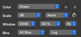
- Change the following settings in the right-hand sidebar that appears with the spectrogram as follows (screenshot):
- Window: 2048 50% 8x
- Bins: All Bins Log
- Other settings can be left unchanged.
- Add new layers with additional analysis.
- Go to Transform > Analysis by maker > Matthias Mauch > pYIN: smoothed pitch track; hit “OK” and just use the default settings. If needed, change the color of the plot to something that will stand out against the spectrogram.
- Go to Transform > Analysis by maker > libxtract > A–S > RMS Amplitude. Change the Window increment setting to 4096; hit “OK” to generate the analysis. On the bottom-right of the property boxes (the right sidebar), toggle off “Show”, so that the RMS amplitude graph is hidden instead of overlaid on the spectrogram.
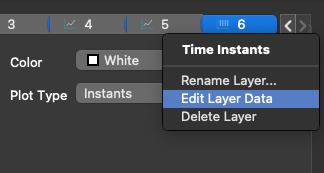
- Go to Layer > Add new time instants layer. Use this to add annotations to the spectrogram that orient us within the form, as follows:
- Refer to the lyrics (uploaded on Teams). Every four lines or so, there is a double-space between lyrics. This indicates different sections of the song.
- For each new section, add a time instant by using the Draw tool. It may help to zoom in enough so that you can visually see where new sections start.
- Once you’ve entered all the time instants, go to the property boxes (the right sidebar) and right-click on the tab for the Time Instants layer and select Edit layer data (screenshot). In the popup window, replace “New Point” with the first word(s) of the lyrics in that section—enough to distinguish the sections and get you oriented.
- Finally, go to File > Export image file. Enter a filename to upload to your homework folder (as a reminder please begin your filename with
9(the current week number); after that I don’t care what the file name is). After you confirm your file name, another dialog box will appear; select the option to export the whole pane. - Upload your PNG file to your homework submit folder.
- Save your Sonic Visualiser session by going to File > Save session. Name it whatever you like and save it somewhere you will be able to easily locate it again. You will need this file to do your homework next week.
Week 10 (Mar 18)
Reading due Tue, Mar 19
Provenzano 2018, Malawey 2020
Discussion leaders: Stephen Gliatto, Rui Tang
Assignment due Fri, Mar 22
This homework assignment will continue to build on the Sonic Visualiser session you created last week, so begin by loading your Sonic Visualiser session. (If you lost your file, redo the assignment from last week…!)
Using Sonic Visualiser as an aid, create an analysis similar to Duguay’s Example 18. “MOVE” has two singers, whose vocals I’d like you to analyze separately: Beyoncé and Grace Jones. If you don’t already know how to distinguish their voices, just listen to a track by each of them—they are pretty different so I don’t think you’ll need much training.
- Open your Sonic Visualiser session from last week.
- I have uploaded a template chart to Teams, titled
duguay-template.xlsx. Download a copy of the chart (please do not edit the one on Teams) to record your analysis. - Export both your Time Instants layer and your RMS Amplitude as CSV files by going to File > Export annotation layer. Open both files.
- Create a row for each section of the song indicated in the lyrics file. Break out your analysis into these different sections. You might find it useful to use your Time Instants data for this.
- For width, environment, and layering, you will analyze through aural analysis (close listening) of the isolated vocals. The spectrogram may help you navigate the recording and attend to certain features, but there are no special tools in Sonic Visualiser to do the work for you.
- For pitch range, because Beyoncé and Grace Jones sometimes sing together, the Smoothed Pitch Track will not be totally accurate, but it is helpful.
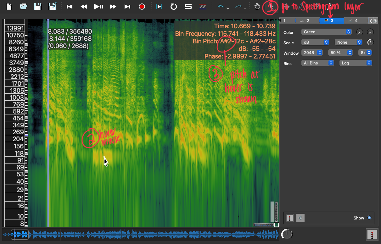
- Listen closely to the isolated vocal track while watching the spectrogram + Smoothed Pitch Track overlay.
- When it seems like the Smoothed Pitch Track missed the fundamental, temporarily hide it by toggling off the Show button in the bottom right of the property boxes; then, when you hover over the correct fundamental on the spectrogram, you should see a box pop up on the top right of the spectrogram that shows the frequency at the point your mouse is over (screenshot).
- For each section, write down the highest and lowest pitch, separated by vocalist.
- For prominence, you will have to export some data generated through Sonic Visualiser plugins and do some math with Excel.
- Prominence needs data from the full audio track (not just the isolated vocals). Start a new Sonic Visualiser session and import the complete audio for “MOVE”.
- Go to Transform > Analysis by maker > libxtract > A–S > RMS Amplitude. Change the Window increment setting to 4096; hit “OK” to generate the analysis.
- Export the RMS Amplitude layer as you did last week. Make sure you title the file something distinct from the other RMS amplitude file you generated with the isolated vocals.
- In
duguay-template.xlsx, open the second tab, titledprominence calculation. - Paste the data from Time Instants into all three of the empty tables. Select those cells you just pasted, and change their background to yellow (this makes them easier to find in the next few steps).
- Paste the data from the isolated RMS Amplitude into the gray empty table, underneath the highlighted Time Instants cells, so that everything is in one table.
- Paste the data from the complete RMS Amplitude into the blue empty table, underneath the highlighted Time Instants cells, so that everything is in one table.
- In both tables, click the little arrow on the header cell titled
time (seconds)and sort the data from smallest to largest. The highlighted cells with form labels will now be properly distributed through the column of data, dividing the data up into sections. - To calculate the average RMS amplitude of a section, go into the corresponding cell in the yellow table and type
=average(and then use your mouse to click and drag to select all the cells in a section. - Finally, the last column in the yellow table will calculate the prominence according to the formula laid out by Duguay, using the formula
=([@[isolated avg]]/[@[complete avg]])*100. This number is what you would enter in your summary table, on the other tab of the Excel sheet. - Once you are (finally…) all done, go to File > Export > PDF. Whew!
- Write a tiny bit of interpretation of the Summary table you created. Use Duguay’s discussion of Example 18 as a model for your own analysis. You might compare how each singer is treated, how the vocal timbre is different in different sections, or something else. Just a couple sentences is plenty—I know you did a lot of work! Export this as a PDF too.
- Combine your two PDFs into one…
- Title your PDF with something beginning with
10(the week number). Upload to your homework submit folder.